🌊 3. Fourier Series for Functions with Period 2π | A key to conquer the (open source) world.

Learn how to compute Fourier series for functions with period 2π. This step-by-step tutorial explains coefficient formulas, orthogonality, the role of \( \frac{a_0}{2} \) and convergence using clear visuals and intuition.

Note: References (2.2.x) are explained in 📐 2. Fourier Series General Concepts.

⚙️ 3.1 Formal treatment — computing the coefficients

Suppose the function \( f(x) \), with period \( 2\pi \), is represented by the series

\[f(x)=\frac{a_{0}}{2}+\sum_{n=1}^{\infty }(a_{n}\cos(nx)+b_{n}\sin(nx))\quad(3.1.1 )\]

Then the coefficients can formally be determined as follows.

• 📏 \( a_{0} \) Finding the constant term \( a_{0} \)

If we integrate both sides of (3.1.1) over one period \( 2\pi \), and assume that the integral \( \int_{}^{} \) and the sum \( \sum_{}^{} \) may be interchanged, we obtain

\( \int_{-\pi}^{\pi}f(x)dx= \\ \frac{a_{0}}{2}
\underbrace{
\int_{-\pi}^{\pi}dx}_{=2\pi\text{ (Hint 1)}}
+\sum_{n=1}^{\infty }\left[ a_{n}
\underbrace{
\int_{-\pi}^{\pi}\cos(nx)dx}_\text{= 0 (See Hint 2)}
+b_{n}
\underbrace{
\int_{-\pi}^{\pi}\sin(nx)dx}_{\substack{\text{= 0 odd integrand}\\\text{over symmetric limits}}}
\right] \)

Hint 1: \( \int_{-\pi}^{\pi}1dx= (\pi - (-\pi))=2\pi \)

Hint 2:

Positive and negative parts cancel over a full period. \( \int_{-\pi}^{\pi}\cos(kx)\,dx = 0 \quad (k \ne 0) \)

As a result: \[ a_{0}=\frac{1}{\pi}\int_{-\pi}^{\pi}f(x)dx\quad(3.1.2 ) \]

• ✖️ ∫ cos Finding the Cosine Coefficients

If we multiply both sides of (3.1.1) by \( \cos(mx) \) and then integrate both sides over one period \( 2\pi \), assuming again that \( \int_{}^{} \) and \(\sum_{}^{} \) may be interchanged, we obtain

\( \int_{-\pi}^{\pi}f(x)cos(mx)dx =\frac{a_{0}}{2}
\underbrace{
\int_{-\pi}^{\pi}\cos(mx)dx}_{\text{=0 (See Hint 2)}}
+\\ \sum_{n=1}^{\infty }\left[ a_{n}
\underbrace{
\int_{-\pi}^{\pi}\cos(nx)\cos(mx)dx}_{\substack{
(2.2.3) \quad
\begin{cases}
0 & n \neq m \\
\pi & n=m>0 \\
2\pi & n=m=0
\end{cases}}
}
+b_{n}
\underbrace{
\int_{-\pi}^{\pi} \sin(nx)\cos(mx)dx }_\text{= 0 (2.2.1)}
\right] \)

On the right-hand side only the second term remains. For this term the condition \( (n=m=0) \) is not possible because the summation starts at \( (n=1) \). During the summation all terms with \( (n \neq m) \) are 0 and disappear. The only remaining term is \( (n = m \gt 0) \).

Therefore we obtain

\[ a_{m}=\frac{1}{\pi}\int_{-\pi}^{\pi}f(x)\cos(mx)dx\quad(3.1.3 ) \]

• ✖️ ∫ sin Finding the Sine Coefficients

If we multiply both sides of (3.1.1) by \( \sin(mx) \) and then integrate both sides over one full period \( 2\pi \), we can isolate the coefficient \(b_{m} \).

Assuming that we are allowed to swap the sum and the integral, we obtain:

\( \int_{-\pi}^{\pi}f(x)sin(mx)dx =\frac{a_{0}}{2}
\underbrace{
\int_{-\pi}^{\pi}\sin(mx)dx}_{\text{=0 (See Hint 3)}}
+\\ \sum_{n=1}^{\infty }\left[ a_{n}
\underbrace{
\int_{-\pi}^{\pi}\cos(nx)\sin(mx)dx}
_\text{= 0 (2.2.1)
}
+b_{n}
\underbrace{
\int_{-\pi}^{\pi} \sin(nx)\sin(mx)dx }
_{\substack{
(2.2.2) \quad
\begin{cases}
0 & n \neq m \\
\pi & n=m>0 \\
0 & n=m=0
\end{cases}}
}
\right] \)

Hint 3:

\( \sin(mx) \) is an odd function:

\[ \sin(-mx)=-\sin(mx) \]

For any odd function:

\[ \int_{-a}^{a} f(x)\,dx = 0 \]

So the positive area cancels the negative area.

On the right-hand side only the third term remains. For this term the condition \( (n = m = 0) \) is not possible because the summation starts at \( (n=1) \). During the summation all terms with \( (n \neq m) \) are 0 and disappear. The only remaining term is \( (n = m \gt 0) \).

Therefore we obtain:

\[ b_{m}=\frac{1}{\pi}\int_{-\pi}^{\pi}f(x) \sin(mx) dx\quad(3.1.4) \]

📘 Definition — Fourier Series

This definition bundles the above knowledge.

Let \( f(x) \) be a function with period \( 2\pi \).

The Fourier series associated with \( f(x) \) is then defined as:

\[ \frac{a_{0}}{2}+ \sum_{n=1}^{\infty}\left( a_{n} \cos(nx) + b_{n} \sin(nx) \right) \quad(3.1.1) \]

The Cosine Fourier coefficients are computed using the following formula:

\[ a_{n} = \frac{1}{\pi}\int_{-\pi}^{\pi}f(x)\cos(nx)\,dx \quad(n=0,1,2,\cdots ) \quad(3.1.5) \]

The Sine Fourier coefficients are computed using the following formula:

\[ b_{n} = \frac{1}{\pi}\int_{-\pi}^{\pi}f(x)\sin(nx)\,dx\quad(n=1,2,3,\cdots ) \quad(3.1.6) \]

💡 Remarks (Important!)

1️⃣ Why do we use \( \frac{a_0}{2} \) instead of \( a_{0} \) in the Fourier series equation?

In a Fourier series, we write:

\[f(x)=\frac{a_{0}}{2}+\sum_{n=1}^{\infty }(a_{n}\cos(nx)+b_{n}\sin(nx))\quad(3.1.1 )\]

At first glance, it might seem more natural to just write \( a_{0} \).

So why do we divide it by 2?

Step 1 — What does \( a_{0} \) represent?

The coefficient is defined as:

\[ a_{0}=\frac{1}{\pi}\int_{-\pi}^{\pi}f(x)dx \]

But the average value of a function over \( (-\pi,\pi) \)is:

\[ \frac{1}{2\pi}\int_{-\pi}^{\pi}f(x)dx \]

So: \( a_{0} \) = 2 × (average value)

👉 This means \( a_{0} \) is twice as large as the constant we actually need.

Step 2 — Fixing the size

To get the correct constant term, we divide by 2:

\[ \frac{a_{0}}{2}=\frac{1}{2\pi}\int_{-\pi}^{\pi}f(x)dx \]

✅ Now it equals the true average of the Fourier function.

Step 3 — Why not just change the formula instead?

We could redefine \( a_{0} \), but then:

the formula for \( a_{n} \) would be different for \( n=0 \) and \( n\ge 1 \)
we would lose one clean, consistent formula:

\[ a_{n}=\frac{1}{\pi}\int_{-\pi}^{\pi}f(x)\cos(nx)dx\quad\text{(works for all }n\ge 0) \]

Using \( \frac{a_0}{2} \) keeps everything uniform.

Step 4 — Why is \( n=0 \) special?

\( \cos(0x)=1 \to \) gives a constant term
\( \sin(0x)=0 \to \)gives nothing

So:

the constant part comes only from cosine
we pull it out of the summation by starting at \( n=1 \) and write it separately as \( \frac{a_0}{2} \)

\[f(x)=\frac{a_{0}}{2}+\sum_{n=1}^{\infty }(a_{n}\cos(nx)+b_{n}\sin(nx))\quad(3.1.1 )\]

Additional advantage:

The formula for the coefficients are kept consistent for all n — including \( n = 0 \).

The cosine coefficients are defined as:

\[ a_{n} = \frac{1}{\pi}\int_{-\pi}^{\pi}f(x)\cos(nx)\,dx \quad(n=0,1,2,\cdots ) \quad(3.1.5) \]

Now look at what happens when \( n = 0 \):

\( \cos(0x) = 1 \)
So:

\[ a_{0}=\frac{1}{\pi}\int_{-\pi}^{\pi}f(x)dx\quad(3.1.2 ) \]

This gives the average value (up to a factor) of the Fourier function.

Bottom line: Using \( \frac{a_0}{2} \):

keeps the formulas symmetric
avoids treating \( a_{0} \) differently
lets one single formula for \( a_{n} \) work for all \( n\ge 0 \)

One sentence intuition:

We use \( \frac{a_0}{2} \) so the constant term fits neatly into the same pattern as all the other cosine terms, without special exceptions.

2️⃣ A note on rigor (important but subtle)

The method we used is not fully rigorous yet.

We assumed that:

A Fourier series representation of \( f(x) \) existed (3.1.1).
We are allowed to swap summation and integration during the calculation of the coefficients.

These assumptions are not automatically true.

👉 Therefore, in a complete theory, we must specify conditions on \( f(x) \) that guarantee:

the Fourier series exists
the series actually represents the function

This is one of the most difficult parts of Fourier theory, so we usually state the result as a theorem called the Dirichlet Conditions (often without proof at first).

🧠 3.2 Theorem: Dirichlet Conditions

If:

\( f \) is defined on the interval \( ]-\pi,\pi[ \), possibly except at a finite number of points where both the left-hand and right-hand limits exist.
\( f \) is periodic with period \( 2\pi \).
The interval \( ]-\pi,\pi[ \) can be divided into sub-intervals on which both \( f \) and its derivative \( f' \) are continuous.

Then, the Fourier series (3.1.1), with coefficients given by (3.1.5) and (3.1.6), converges:

to \( f(x) \) at points where \( f \) is continuous, and
to the average of the left-hand and right-hand limits at points of discontinuity.

Remark

The conditions (1), (2), and (3) are sufficient conditions. Most functions encountered in applications satisfy them.

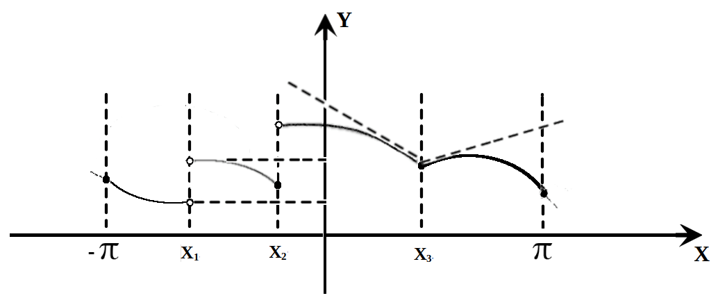
Special Cases Illustrated in the Graph Above:

\( f \) is not defined at \( x_{1} \), the Fourier series converges to \( \frac{f(x_{1}-0)+f(x_{1}+0)}{2} \).
\( f \) is defined at \( x_{2} \) but is discontinuous there, the Fourier series converges to \( \frac{f(x_{2}-0)+f(x_{2}+0)}{2} \) not to \( f(x_{2}) \)!
\( f \) is continuous but not differentiable at \( x_{3} \), the Fourier series converges to \( f(x_{3}) \).

Hint: The meaning of \( \frac{f(x_{n}-0)+f(x_{n}+0)}{2} \):

\(f(x_{n}-0) \): The left-hand limit of the function at \( x_{n} \)
\( \to \) The value \( f(x) \) approaches as \( x\to x_{n} \) from the left.
\(f(x_{n}+0) \): The right-hand limit of the function at \( x_{n} \)
\( \to \) The value \( f(x) \) approaches as \( x\to x_{n} \) from the right.
The whole expression is simply the average of those two values.
Why does this appear?
At a jump discontinuity, the function has two different “sides.” The Fourier series can’t choose one, so it converges to the midpoint between them.

A real life example:

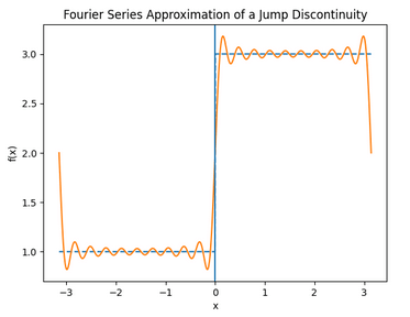
Interpreting the graph:

The dashed line is the original function:
- Left of 0 \( \to \) value = 1
- Right of 0 \( \to \) value = 3
- So there’s a jump at x = 0
The solid curve is the Fourier series approximation.

What to notice 👇

Near most points, the Fourier series follows the function well.
But near the jump at x = 0, it oscillates (this is called the Gibbs phenomenon).
Exactly at the jump, the curve settles around:

\[\frac{1+3}{2}=2 \]

Key Idea: The Fourier series cannot “jump” instantly, because it’s built from smooth sine waves. So at a discontinuity: